3D Genome Browser
2.0 Document
Table of Contents
Getting Started with the 3D
Genome Browser 2.0
Loading
data on the 3D Genome Browser 2.0
Navigating
the 3D Genome Browser 2.0
Exporting
plots from the 3D Genome Browser 2.0, a complete walkthrough
Exploring
the SV Dataset on the 3D Genome Browser 2.0
Notes:
1. To follow along
this tutorial, click along in the order of the numbered circles on the
screenshots.
![]()
2. Certain features
are labelled in alphabetical order.
![]()
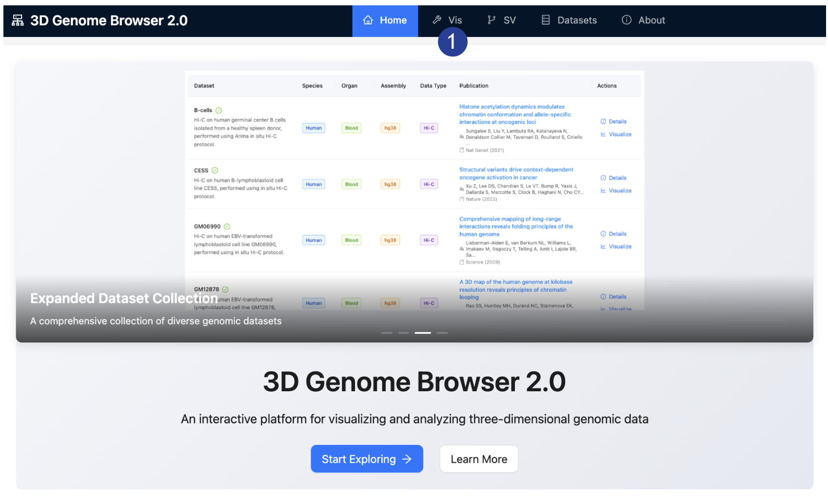
Getting Started
with the 3D Genome Browser 2.0
1.
Load the
browser:
o
Access our
browser at https://3dgenome.fsm.northwestern.edu/
§
Web
supported: Chrome, Firefox, Safari, Edge and More!
2.
On the top
bar: Select the “Vis” tab.
Loading data on
the 3D Genome Browser 2.0
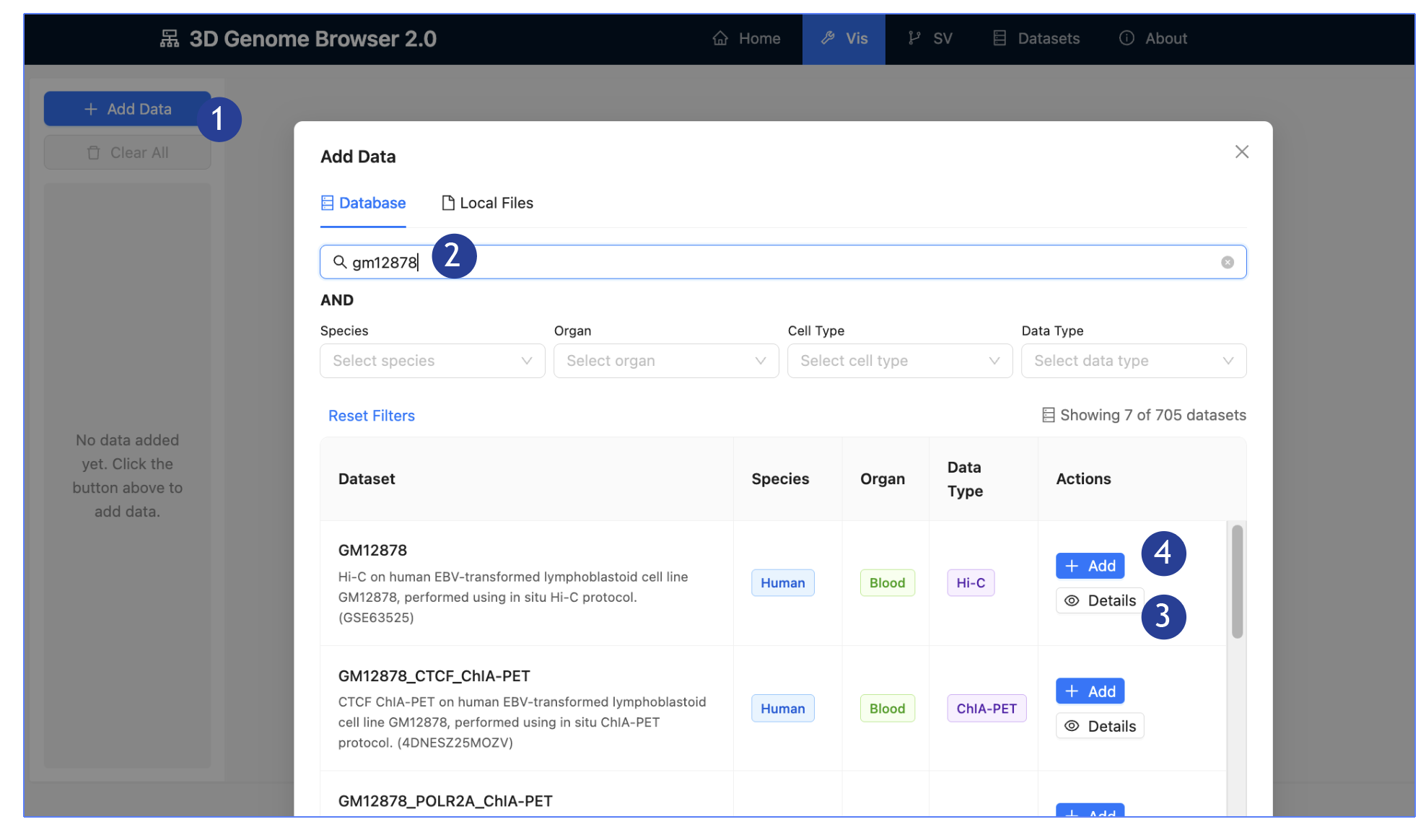
1.
On the Left
Panel: Click “Add Data”, an “Add Data” page will pop-up.
2.
Browse our
hosted data:
o
Search
datasets by the provided search bar
o
Filter
datasets by:
§
Species
§
Organ of
origin
§
Cell type
§
Data type
3.
Click on
Details for a dedicated page detailing the dataset, including metadata,
description and linked publication.
4.
Click “Add”
to add the dataset on interest into the main panel:
o
Multiple
datasets can be visualized at once.
§
Repeat step
one to select another dataset.
o
In this
tutorial, we will visualize GM12878 Hi-C and GM12878 CTCF ChIA-PET.
5.
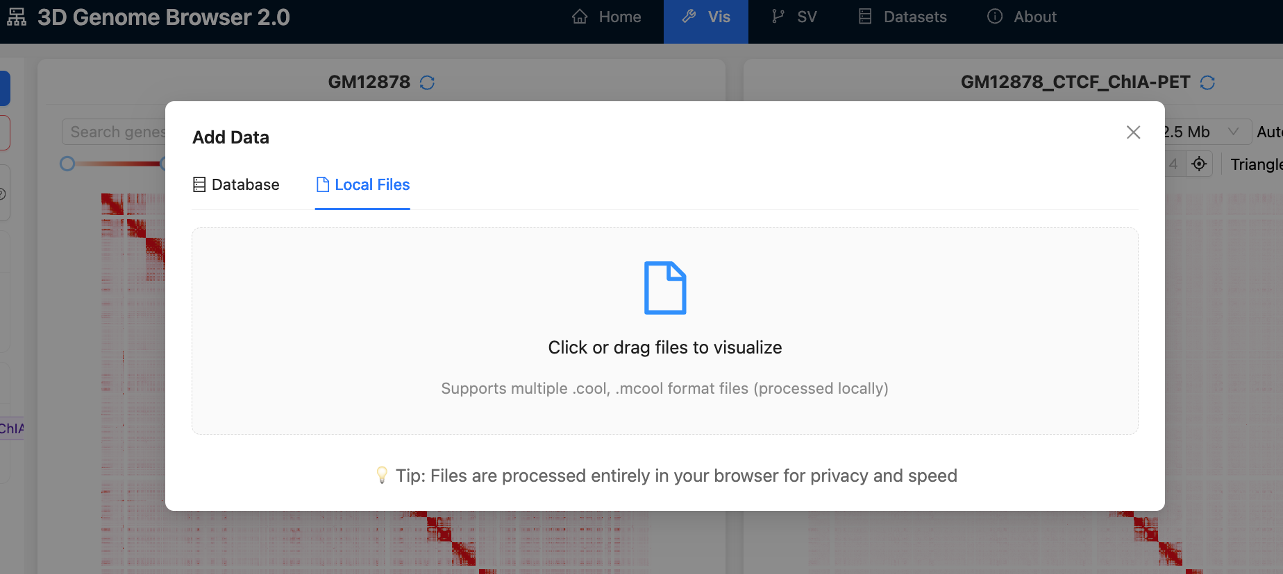
The browser
also supports local files in .cool or
.mcool format
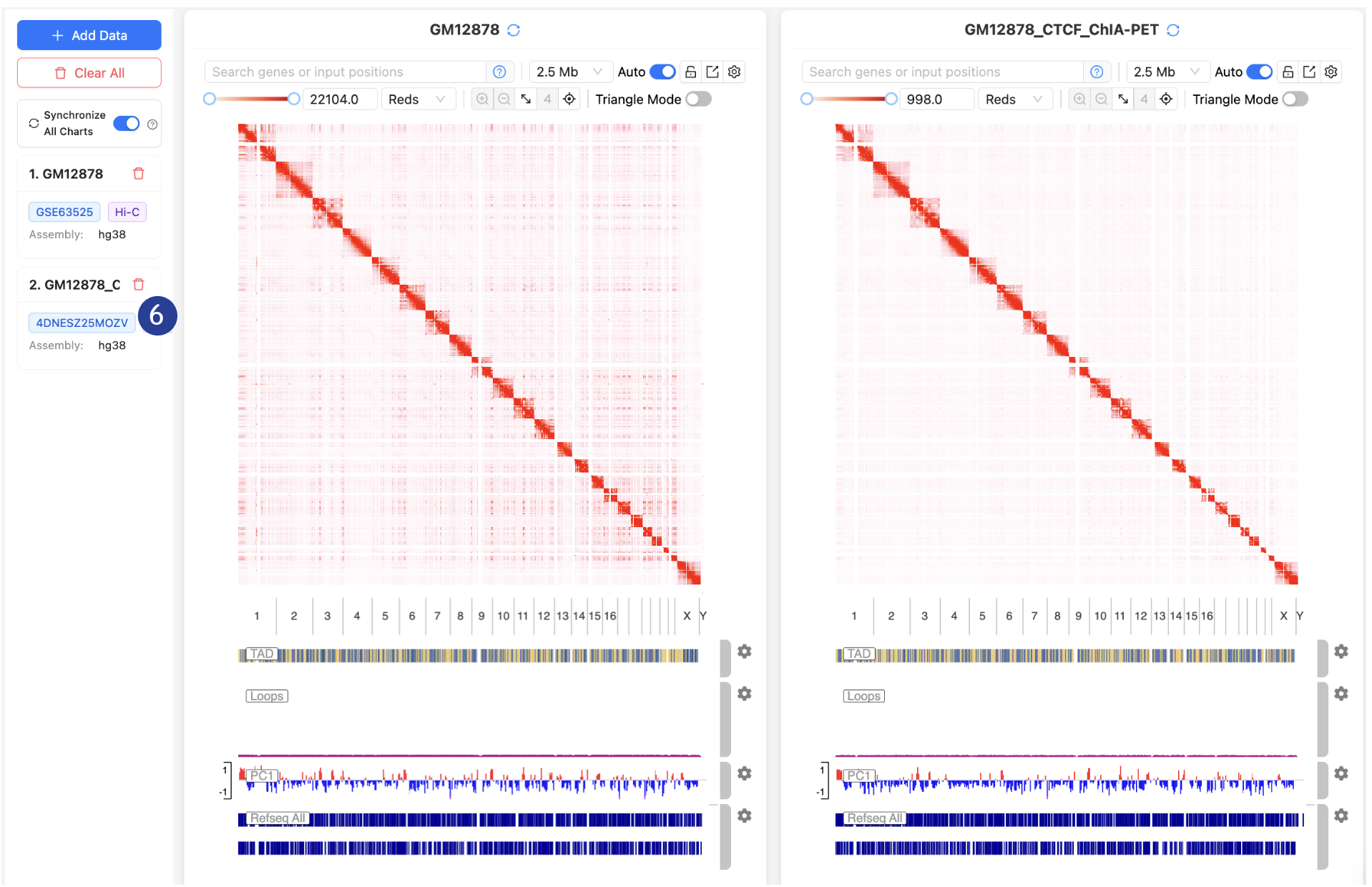
6.
Loaded
datasets can be removed by the trashbin icon
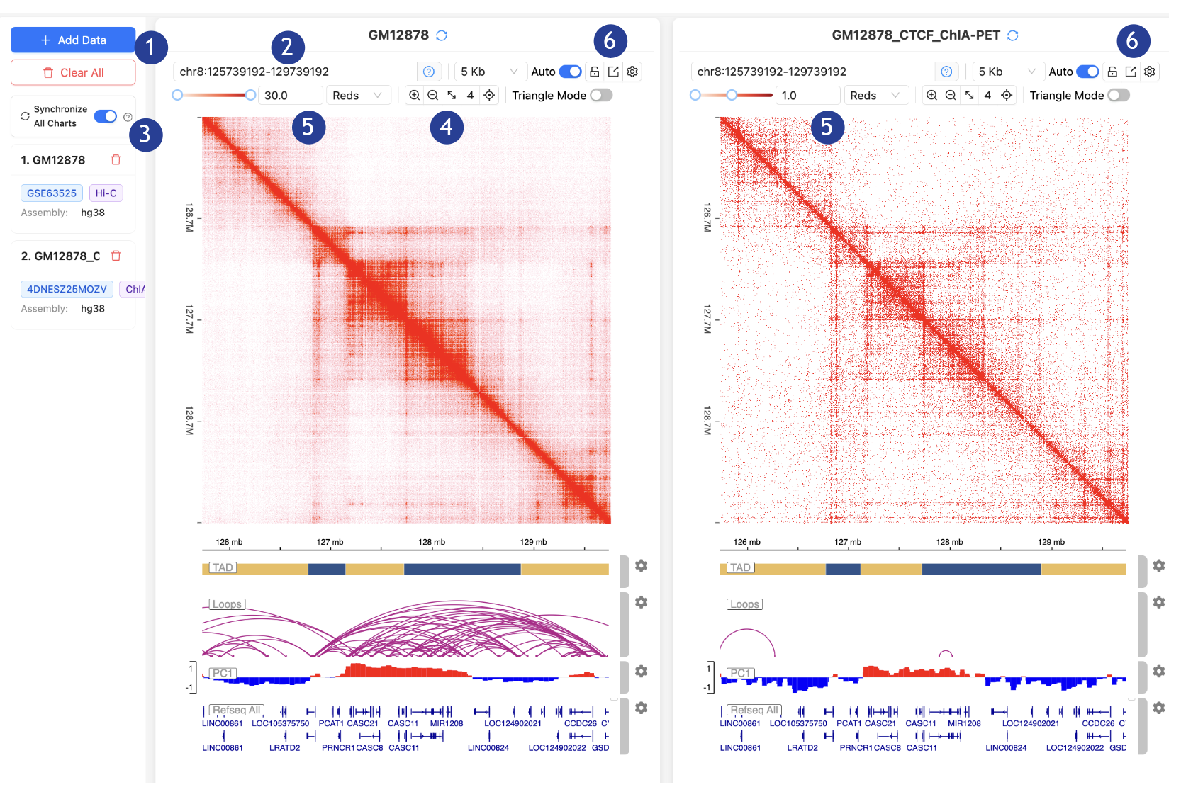
Navigating the
3D Genome Browser 2.0
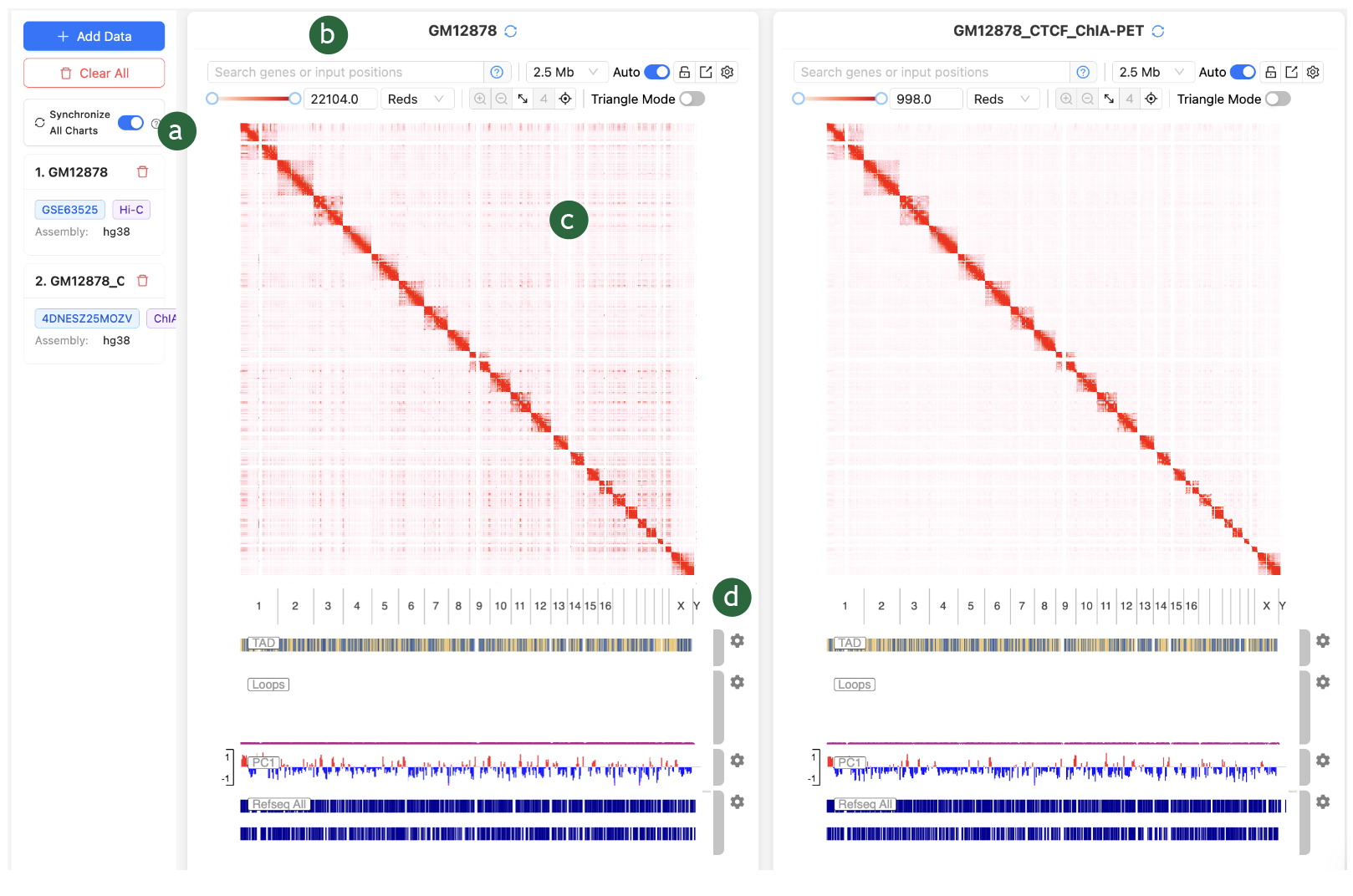
1.
There are 4
key modules in the 3D Genome Browser 2.0:
a)
Data
selection bar, which we have covered in the previous section.
b)
Quick adjust
toolbar
c)
Interactive
Contact Map
d)
Genomic
Track
We
will be covering the b c and d in this section.
2.
The quick
adjust bar contains most of the functions for visualization and analysis:
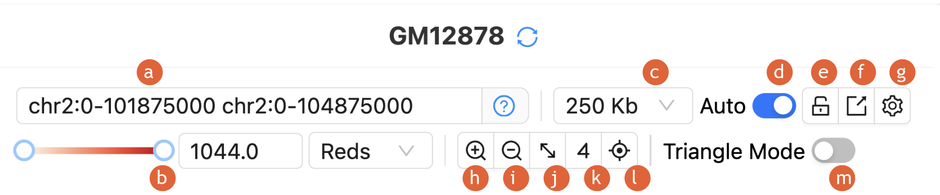
a)
Input
positions/Coordinate search
§
Search by
gene name, chromosome name or genome coordinates
b)
Contact map
color adjustments
§
Different
color scheme available
c)
Set
resolutions
d)
Toggle auto
resolutions
e)
Toggle lock
resolutions
f)
Export plot
§
PNG, SVG
formats available
g)
Data
normalization
§
ICE, Log2
normalization available
h)
Zoom in
i)
Zoom out
j)
Lock
Diagonal (Sync X/Y Axes)
k)
Toggle
Virtual 4C Mode
l)
Toggle
auxiliary line for mouse cursor
m)
Toggle
Triangle mode
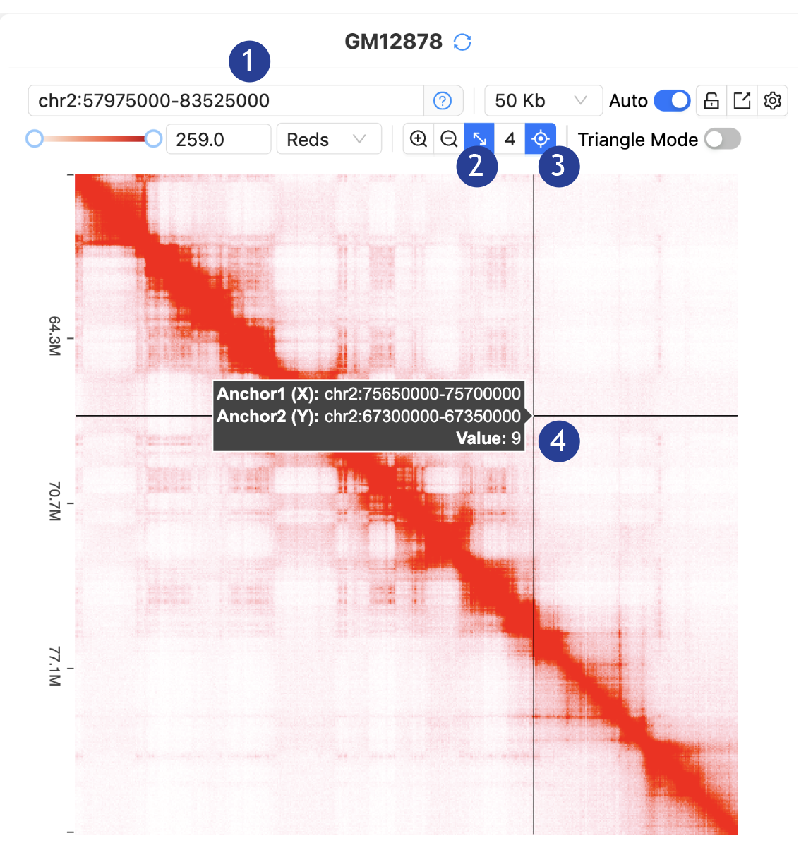
3.
The
Interactive Contact Map allows visualization and interaction:
1.
Paste the
coordinates (chr2:57975000-83525000) in the “Input positions” and hit Enter key
2.
Lock the
diagonal: In the toorbar, click “Lock Diagonal”
3.
Toggle on
the auxiliary line: In the toorbar, click “Auxiliary
Line”
4.
Hoover mouse
cursor on the interactive contact map. Anchor positions and contact values for
any position on the map will be visualized.
5.
Interacting
with the contact map: Dragging will update the coordinates. Double-clicking
will zoom in.
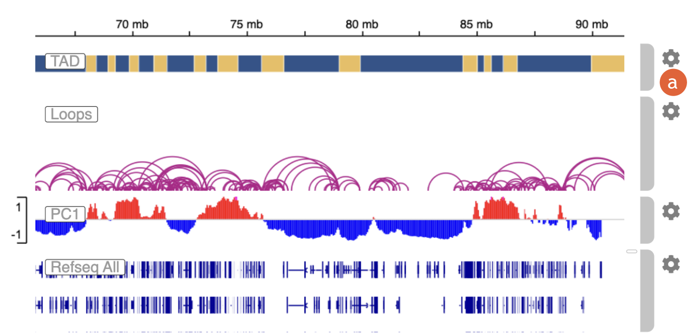
4.
The Genomic
Track module is powered by the Integrative Genomics Viewer (IGV) embeddable
API:
a)
Click on the
gear icon to customize display options
Exporting plots
from the 3D Genome Browser 2.0, a complete walkthrough
1.
Load the
hosted dataset: GM12878 Hi-C and GM12878 CTCF ChIA-PET.
2.
In the
“Input positions” search bar: Type “MYC” and select the first option in the pop-up
bar (MYC chr8:127735434-127742951).
3.
Make sure
the “Synchronize All Charts” is toggled ON.
4.
“Zoom out”
button: Click TWICE.
5.
In the
“Contact Map Color Scale”: Type “30 “in GM12878 Hi-C and hit Enter; Type “1” in
GM12878 CTCF ChIA-PET and hit Enter.
6.
“Export
plot” button: Click on “Export as PNG” for both of the contact maps.
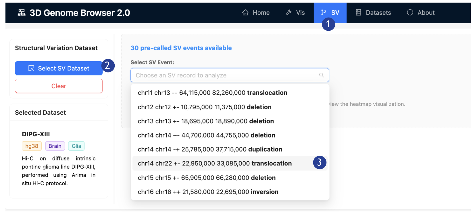
Exploring the
SV Dataset on the 3D Genome Browser 2.0
1. On the top bar: Select the
“SV” tab.
2.
On the Left
Panel: Click “Add Data”, an “Add Data” page will pop-up. Select the dataset
“DIPG-XIII”.
3.
On the
“Select SV Event” dropdown list: Select “chr14 chr22 +- 22,950,000 33,085,000 translocation”
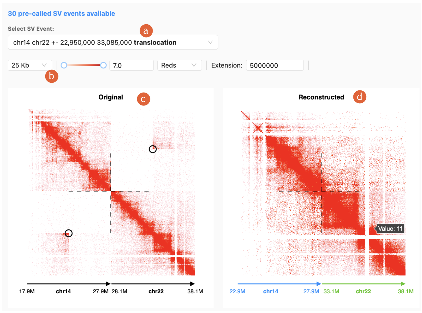
4.
The SV
reconstruction contact map will be generated, with the following features:
a)
“Select SV
Event” dropdown list: select any pre-called SV events
b)
Contact map
color adjustments and resolution adjustments
c)
“Original”
contact map: Contact map before reconstruction, breakpoint highlighted in black
circle
d)
“Reconstructed”
contact map: Computationally modeled after the specified rearrangement, powered
by NeoloopFinder, breakpoint highlighted in dotted
cross
Supplemental
Notes:
Loop calling using Peakachu1
All of our hosted Loop
files are called using Peakachu (v2.3), a supervised
learning software that predicts chromatin loops from genome-wide contact maps.
For all of our hosted datasets, we used the following parameters to perform
loop calling:
--resolution 10000
--model chosen according
to the total intra reads
For more details, please
see: https://github.com/tariks/peakachu
A/B Compartment calling and TAD calling using cooltools2
Both A/B Compartment
calling and TAD calling were performed using cooltools
(v0.8.7) eigs-cis and insulation
functions, respectively. For A/B Compartment calling, either 50kb or 40kb
resolutions were used, whichever lower is available. For TAD calling, either
25kb or 20kb resolutions were used, whichever lower is available; --threshold
0.5 –append-raw-scores; window size was set to 10 times of the resolution
applied.
For more details, please
see: https://cooltools.readthedocs.io/en/latest/index.html
References
1.
Salameh TJ,
Wang X, Song F, Zhang B, Wright SM, Khunsriraksakul
C, Ruan Y, Yue F. A supervised learning framework for chromatin loop detection
in genome-wide contact maps. Nat Commun. 2020 Jul 9;11(1):3428. doi: 10.1038/s41467-020-17239-9
2.
Open2C; Abdennur N, Abraham S, Fudenberg
G, Flyamer IM, Galitsyna
AA, Goloborodko A, Imakaev
M, Oksuz BA, Venev SV, Xiao
Y. Cooltools: Enabling high-resolution Hi-C analysis
in Python. PLoS Comput
Biol. 2024 May 6;20(5):e1012067. doi:
10.1371/journal.pcbi.1012067